Learning to really read query plans
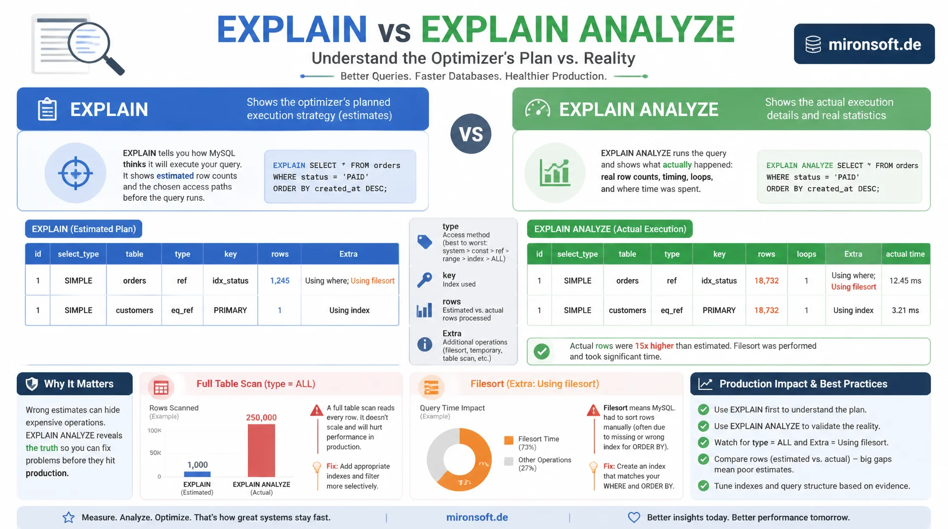
EXPLAIN shows what the optimizer plans, EXPLAIN ANALYZE shows what actually happened. Anyone who correctly interprets type, key, rows and Extra, and compares estimated rows against real execution statistics, finds full table scans and filesorts before they become a problem in production.
Table of contents
- 1. Why reading query plans is a core skill
- 2. The classic EXPLAIN output: type, key and rows
- 3. Correctly interpreting join types
- 4. Decoding the Extra column
- 5. EXPLAIN ANALYZE: real execution statistics
- 6. Estimated versus actual rows: spotting statistics drift
- 7. Hunting down full table scans and filesorts
- 8. EXPLAIN FORMAT=JSON for deep analysis
- 9. Practical workflow: from slow query to fix
- 10. Summary
- 11. FAQ
1. Why reading query plans is a core skill
A query plan is the optimizer's decision on how to execute a query: which indexes are used, in what order tables are joined, and whether sorting happens inside the index or afterward in memory. Anyone who does not read EXPLAIN optimizes queries by gut feeling, and gut feeling regularly misses the mark once data volumes reach the millions. The query plan is the only reliable source of what MySQL actually intends to do for a given query.
In practice, the difference between an index access hitting a few hundred rows and a full table scan over millions of rows decides milliseconds versus seconds of response time. That decision is visible in the query plan long before it becomes a problem in production. The following sections show how to read the classic EXPLAIN output, how EXPLAIN ANALYZE additionally provides real execution numbers, and how to systematically derive optimizations from that.
The critical mistake when reading query plans is treating EXPLAIN as pure confirmation ("an index is used, so everything is fine") instead of as a diagnostic tool. Using an index is necessary but not sufficient for a fast query. Only the interplay of type, rows, and Extra shows whether the query plan is actually efficient.
2. The classic EXPLAIN output: type, key and rows
The type column in the query plan shows the access method, sorted from fast to slow: const, eq_ref, ref, range, index, ALL. const means at most one row is found via a primary or unique key, usually for an ID lookup. ALL means a full table scan where every row is checked. In between sit ref for index accesses with an equality condition and range for range queries over an index.
The key column shows which index was actually used, as opposed to possible_keys, which only lists the theoretically eligible indexes. An empty key value despite a populated possible_keys is a clear warning sign: the optimizer recognized an index as possible but decided against using it, usually because the statistics estimate a full table scan as cheaper.
The rows column is an estimate, not an exact number, based on the table statistics. It states how many rows the optimizer has to search through for this step of the query plan before filter conditions are applied. A low rows value in a JOIN across several tables is critical, because the values can multiply across nested loops and an innocent looking number can quickly become a million-row problem.
EXPLAIN SELECT o.id, c.email FROM orders o
JOIN customers c ON c.id = o.customer_id
WHERE o.status = 2 AND o.created_at > '2026-01-01'\G

*************************** 1. row ***************************
           id: 1
  select_type: SIMPLE
        table: o
         type: range
possible_keys: idx_status_created,idx_customer_id
          key: idx_status_created
      key_len: 4
          ref: NULL
         rows: 1840
        Extra: Using index condition
*************************** 2. row ***************************
           id: 1
  select_type: SIMPLE
        table: c
         type: eq_ref
possible_keys: PRIMARY
          key: PRIMARY
      key_len: 4
          ref: shop.o.customer_id
         rows: 1
        Extra: NULL
3. Correctly interpreting join types
In the query plan of a JOIN, a separate row appears for each involved table, and the order of these rows shows the actual processing order, which does not necessarily match the order in the SQL statement. The optimizer typically chooses to search the table with the lowest estimated row count first and then jump into the next table via an index. An eq_ref for the second table means that for each row of the first table exactly one matching row is found via a unique or primary key, which is a very efficient join type.
A query plan becomes problematic when a later table in the join shows type: ALL, because then a complete scan of that table is performed for every row of the previous table, which compounds multiplicatively. With ten thousand rows from the first table and a full table scan over a hundred thousand rows in the second, the worst case produces billions of checked combinations, even if the final result only has a handful of rows.
The optimizer fundamentally decides the join order itself and ignores the order of tables in the FROM and JOIN clauses of the SQL statement. If you see an unexpected order in the query plan, do not interpret it as a bug but as the result of the optimizer's cost estimate, which in turn depends on current table statistics.
4. Decoding the Extra column
The Extra column contains the most important warning signals in the entire query plan. Using filesort means MySQL cannot deliver the result set sorted via an index and instead performs a separate sort operation in memory or on disk. Using temporary means a temporary table is created for GROUP BY, DISTINCT, or complex subqueries, which causes significant overhead for large intermediate results.
Using index, on the other hand, is a positive signal: all needed columns are read directly from the index without touching the actual table. This is the so called covering index, covered in depth in a dedicated article. Using where shows that after the index access an additional filter condition is checked in the storage engine or server layer, which can mean many unnecessarily read rows when the index has low selectivity.
Multiple entries in the Extra column, separated by semicolons, are normal and describe consecutive processing steps for the same table in the query plan. The combination Using where; Using index, for example, means both a covering index and an additional filter condition are applied inside the index, without the actual table needing to be read.
EXPLAIN SELECT customer_id, COUNT(*) FROM orders
WHERE status = 2
GROUP BY customer_id
ORDER BY COUNT(*) DESC\G

*************************** 1. row ***************************
        table: orders
         type: ref
          key: idx_status
         rows: 48210
        Extra: Using where; Using temporary; Using filesort
-- Using temporary: a temp table is built for GROUP BY
-- Using filesort: the aggregated result is sorted separately afterwards
5. EXPLAIN ANALYZE: real execution statistics
The decisive difference between EXPLAIN and EXPLAIN ANALYZE: EXPLAIN shows a plan that is never executed, while EXPLAIN ANALYZE actually executes the query and measures the real runtimes and row counts per step of the query plan. Since MySQL 8.0.18, EXPLAIN ANALYZE provides a tree shaped output with actual time, giving the actual start time and total duration of each operator in milliseconds, and actual rows for the row count that was really processed.
Because EXPLAIN ANALYZE really executes the query, it should never be used uncontrolled on production UPDATE or DELETE statements without being aware of the side effects. For SELECT queries the risk is low, but with very large result sets EXPLAIN ANALYZE can itself generate noticeable load, because the entire query runs to completion, even if the original query plan only actually asked for a LIMIT of ten rows.
EXPLAIN ANALYZE
SELECT o.id, c.email FROM orders o
JOIN customers c ON c.id = o.customer_id
WHERE o.status = 2 AND o.created_at > '2026-01-01';

-> Nested loop inner join  (cost=612.40 rows=1840) (actual time=0.089..4.812 rows=1793 loops=1)
    -> Index range scan on o using idx_status_created
       (cost=201.20 rows=1840) (actual time=0.061..1.204 rows=1840 loops=1)
    -> Single-row index lookup on c using PRIMARY (id=o.customer_id)
       (cost=0.25 rows=1) (actual time=0.001..0.001 rows=1 loops=1840)
6. Estimated versus actual rows: spotting statistics drift
The most valuable comparison when reading EXPLAIN ANALYZE is estimated versus actual row count. If both values differ by more than a factor of ten, this is called statistics drift: the table statistics used by the optimizer are stale, and the chosen query plan is based on wrong assumptions about data distribution. This often leads to a suboptimal join order or the wrong choice between index access and full table scan.
Statistics drift typically arises after large bulk inserts, after deleting large amounts of data, or simply through the persistent nature of InnoDB statistics, which are not automatically recalculated on every change by default. An ANALYZE TABLE after significant data changes refreshes the statistics and is often the simplest fix when EXPLAIN ANALYZE shows a marked deviation between estimated and actual row counts.
-- Before: optimizer estimate is far off from reality
EXPLAIN ANALYZE SELECT id FROM orders WHERE status = 2;
-> Index range scan on orders using idx_status
   (cost=201.20 rows=1840) (actual time=0.05..38.220 rows=48210 loops=1)
-- estimated 1840 rows, actually 48210 -- statistics drift, factor 26

ANALYZE TABLE orders;
-- Table statistics rebuilt from a fresh sample of the table

-- After: estimate matches reality much more closely
EXPLAIN ANALYZE SELECT id FROM orders WHERE status = 2;
-> Index range scan on orders using idx_status
   (cost=4820.10 rows=47990) (actual time=0.05..38.010 rows=48210 loops=1)
7. Hunting down full table scans and filesorts
A systematic way to find problematic query plans in an existing application goes through the slow query log combined with pt-query-digest or the performance schema table events_statements_summary_by_digest. Both identify the most frequent and most expensive queries, which you then examine specifically with EXPLAIN ANALYZE. Full table scans show up as type: ALL combined with a high rows number, filesorts as Using filesort in the Extra column.
Not every full table scan is a problem: for small lookup tables with a few hundred rows, a scan is often faster than the overhead of an index access. The decisive question is always the absolute row count combined with query frequency. A filesort over twenty rows in a rarely executed admin query is uncritical, the same filesort over a million rows on every product page request of a shop is an acute performance killer.
A pragmatic threshold for initial prioritization: queries examining more than ten thousand rows according to rows, combined with more than a hundred executions per minute according to the performance schema, deserve first attention. Everything below that can usually wait until the bigger issues in the query plan are fixed.
8. EXPLAIN FORMAT=JSON for deep analysis
For complex query plans with multiple subqueries, derived tables, or window functions, EXPLAIN FORMAT=JSON provides additional details missing from the classic table form, such as estimated cost per step (cost_info), the sort algorithms used, and the exact structure of nested queries. Combined with ANALYZE as EXPLAIN ANALYZE FORMAT=JSON, you get the most complete available view of a query plan, including real runtimes per nested element.
The JSON format is especially suited for automated evaluation, for example when query plans need to be checked against thresholds for rows or cost in CI pipelines, to catch regressions from new migrations early, before a query becomes slow in production.
EXPLAIN FORMAT=JSON SELECT id FROM orders WHERE status = 2\G
{
  "query_block": {
    "select_id": 1,
    "cost_info": { "query_cost": "4820.10" },
    "table": {
      "table_name": "orders",
      "access_type": "ref",
      "possible_keys": ["idx_status"],
      "key": "idx_status",
      "rows_examined_per_scan": 47990,
      "filtered": "100.00"
    }
  }
}
9. Practical workflow: from slow query to fix
The practical workflow starts with the slow query log to identify the query with the highest cumulative runtime. Next comes EXPLAIN ANALYZE for the exact query with realistic parameters, since a query plan can differ depending on the values passed in. First check type for ALL or index as a warning sign, then Extra for Using filesort or Using temporary, and finally compare estimated with actual rows for statistics drift.
After diagnosis comes the targeted fix: a new composite index, a query rewrite, or ANALYZE TABLE for stale statistics. The fix is verified again with EXPLAIN ANALYZE, to make sure the actual runtime improved, not just that the theoretical query plan looks better. This repetition matters because a new index can, in rare cases, produce a different, equally suboptimal plan.
For quick prioritization, an overview of the most important signals in the query plan helps, sorted by severity.
| Signal in the query plan | Meaning | Severity | Typical action |
|---|---|---|---|
| type: ALL | Full table scan | High on large tables | Add a matching composite index |
| Using filesort | Sort happening outside the index | Medium to high | Align index order with ORDER BY |
| Using temporary | Temporary table for GROUP BY/DISTINCT | Medium to high | Index the GROUP BY columns |
| key: NULL despite possible_keys | Index discarded despite being eligible | Medium | ANALYZE TABLE, check statistics |
| Using index | Covering index, no table access | Positive | None, keep as is |
These signals do not replace a full analysis but give a quick first assessment of which queries from a long slow query log should be examined first. Combined with EXPLAIN ANALYZE and actual row counts, a complete picture of the query plan emerges.
It is also important to re-check the query plan after every schema change. A new composite index can speed up existing queries but can also cause the optimizer to suddenly pick a less favorable plan for a different query, because the relative costs between several possible indexes have shifted. A recurring look at EXPLAIN ANALYZE after every index change belongs to the workflow just as much as the initial diagnosis.
Mironsoft
Query analysis, EXPLAIN audits, and MySQL performance tuning
Query plans nobody on your team actually reads?
We analyze your slowest queries with EXPLAIN ANALYZE, uncover full table scans and filesorts, and translate the results into concrete index and query changes.
Slow query analysis
Prioritize the most expensive queries from logs and performance schema
EXPLAIN workshop
Your team learns to read and assess query plans themselves
Statistics monitoring
Automated checks for statistics drift and stale plans
10. Summary
The query plan is the only reliable source for how MySQL actually executes a query. type, key, and rows show the access method and estimated row count, while the Extra column with Using filesort and Using temporary exposes the most expensive additional operations. EXPLAIN ANALYZE supplements these estimates with real runtimes and actual row counts per step, and makes statistics drift visible.
The systematic workflow of slow query log, EXPLAIN ANALYZE, and targeted action, followed by re-verification, turns reading query plans from an art into a repeatable process. Anyone who confidently interprets type, key, rows, and Extra finds full table scans and filesorts long before they cause timeouts in production.
In the end, the habit that pays off most is running every new or changed query through EXPLAIN ANALYZE once before deployment. A query plan that looks unremarkable in a development system with a few thousand test rows can behave completely differently at millions of rows in production, especially when statistics or data distribution diverge significantly.
EXPLAIN ANALYZE, reading query plans: the essentials
Check type and key
type: ALL and an empty key despite possible_keys are the first warning signs in a query plan.
Read the Extra column
Using filesort and Using temporary show expensive extra operations outside the index.
Use EXPLAIN ANALYZE
Real actual time and actual rows instead of pure estimates, but with care on production writes.
Spot statistics drift
Fix large deviations between estimated and actual rows with ANALYZE TABLE.